
如果你是一名计算机专业的学生,有对图论有基本的了解,那么你一定知道一些著名的最优路径解,如Dijkstra算法、Bellman-Ford算法和a*算法(A-Star)等。
这些算法都是大佬们经过无数小时的努力才发现的,但是现在已经是人工智能的时代,强化学习算法能够为我们提出和前辈一样好的解决方案吗?
本文中我们将尝试找出一种方法,在从目的地a移动到目的地B时尽可能减少遍历路径。我们使用自己的创建虚拟数据来提供演示,下面代码将创建虚拟的交通网格:
import networkx as nx

# Create the graph object
G=nx.Graph()

# Define the nodes
nodes=['New York, NY', 'Los Angeles, CA', 'Chicago, IL', 'Houston, TX', 'Phoenix, AZ', 'Dallas, TX', 'Miami, FL']

# Add the nodes to the graph
G.add_nodes_from(nodes)

# Define the edges and their distances
edges=[('New York, NY', 'Chicago, IL',{'distance': 790}),
         ('New York, NY', 'Miami, FL',{'distance': 1300}),
         ('Chicago, IL', 'Dallas, TX',{'distance': 960}),
         ('Dallas, TX', 'Houston, TX',{'distance': 240}),
         ('Houston, TX', 'Phoenix, AZ',{'distance': 1170}),
         ('Phoenix, AZ', 'Los Angeles, CA',{'distance': 380}),
         ('Los Angeles, CA', 'Dallas, TX',{'distance': 1240}),
         ('Los Angeles, CA', 'Chicago, IL',{'distance': 2010})]

# Add the edges to the graph
G.add_edges_from(edges)
运行起来没有报错,但是我们不知道数据是什么样子的,所以让我们先进行可视化,了解数据:
import matplotlib.pyplot as plt

# set positions for the nodes (optional)
pos=nx.spring_layout(G)

# draw the nodes and edges
nx.draw_networkx_nodes(G, pos, node_color='lightblue', node_size=500)
nx.draw_networkx_edges(G, pos, edge_color='gray', width=2)

# draw edge labels
edge_labels=nx.get_edge_attributes(G, 'weight')
nx.draw_networkx_edge_labels(G, pos, edge_labels=edge_labels)

# draw node labels
node_labels={node: node.split(',')[0]for node in G.nodes()}
nx.draw_networkx_labels(G, pos, labels=node_labels)

# show the plot
plt.axis('off')
plt.show()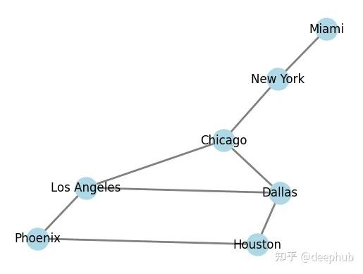
我们有了一个基本的节点网络。但是这感觉太简单了。对于一个强化学习代理来说,这基本上没有难度,所以我们增加更多的节点:
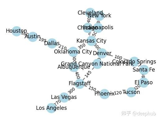
这样就复杂多了,但是它看起来很混乱,比如从New York 到 Arizona就可能是一个挑战。
我们这里使用最常见且通用的Q-Learning来解决这个问题,因为它有动作-状态对矩阵,可以帮助确定最佳的动作。在寻找图中最短路径的情况下,Q-Learning可以通过迭代更新每个状态-动作对的q值来确定两个节点之间的最优路径。
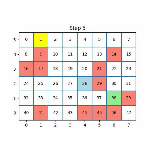
上图为q值的演示。
下面我们开始实现自己的Q-Learning
import networkx as nx
import numpy as np

def q_learning_shortest_path(G, start_node, end_node, learning_rate=0.8, discount_factor=0.95, epsilon=0.2, num_episodes=1000):
 """
    Calculates the shortest path in a graph G using Q-learning algorithm.

    Parameters:
        G (networkx.Graph): the graph
        start_node: the starting node
        end_node: the destination node
        learning_rate (float): the learning rate (default=0.8)
        discount_factor (float): the discount factor (default=0.95)
        epsilon (float): the exploration factor (default=0.2)
        num_episodes (int): the number of episodes (default=1000)

    Returns:
        A list with the shortest path from start_node to end_node.
    """
我们的输入是整个的图,还有开始和结束的节点,首先就需要提取每个节点之间的距离,将其提供给Q-learning算法。
# Extract nodes and edges data
    nodes=list(G.nodes())
    num_nodes=len(nodes)
    edges=list(G.edges(data=True))
    num_edges=len(edges)
    edge_distances=np.zeros((num_nodes, num_nodes))
 for i, j, data in edges:
        edge_distances[nodes.index(i), nodes.index(j)]=data['weight']
        edge_distances[nodes.index(j), nodes.index(i)]=data['weight']
创建一个Q-table ,这样我们就可以在不断更新模型的同时更新值。
# Initialize Q-values table
    q_table=np.zeros((num_nodes, num_nodes))

 # Convert start and end node to node indices
    start_node_index=nodes.index(start_node)
    end_node_index=nodes.index(end_node)
下面就是强化学习算法的核心!
# Q-learning algorithm
 for episode in range(num_episodes):
        current_node=start_node_index
        print(episode)
 while current_node !=end_node_index:
 # Choose action based on epsilon-greedy policy
 if np.random.uniform(0, 1) < epsilon:
 # Explore
                possible_actions=np.where(edge_distances[current_node,:]> 0)[0]
 if len(possible_actions)==0:
                    break
                action=np.random.choice(possible_actions)
 else:
 # Exploit
                possible_actions=np.where(q_table[current_node,:]==np.max(q_table[current_node,:]))[0]
 if len(possible_actions)==0:
                    break
                action=np.random.choice(possible_actions)

 # Calculate reward and update Q-value
            next_node=action
            reward=-edge_distances[current_node, next_node]
            q_table[current_node, next_node]=(1 - learning_rate) * q_table[current_node, next_node]+ learning_rate * (reward + discount_factor * np.max(q_table[next_node, :]))
 # Move to next node
            current_node=next_node
 if current_node==end_node_index:
                break
    print(q_table)
这里需要注意的事情是,我们鼓励模型探索还是利用一个特定的路径。

大多数强化算法都是基于这种简单的权衡制定的。 过多的探索的问题在于它可能导致代理花费太多时间探索环境,而没有足够的时间利用它已经学到的知识,可能导致代理采取次优行动并最终无法实现其目标。 如果探索率设置得太高,代理可能永远不会收敛到最优策略。但是如果探索率设置得太低,代理可能会陷入次优策略。 所以,需要在探索和利用之间取得平衡,确保代理进行足够的探索以了解环境,同时利用其知识来最大化回报。

而强化学习中过多利用的问题会使代理陷入次优策略,无法发现可能更好的动作或状态。 即使有更好的选择,代理也可能对其当前的政策过于自信。 这被称为“漏洞利用陷阱”或“局部最优”问题,代理无法从次优解决方案中逃脱。 在这种情况下,探索有助于发现更好的策略和避免“局部最优”。
回到我们的代码,我们需要检查Q-table ,并确保可以从中提取出最短路径。
# Extract shortest path from Q-values table
    shortest_path=[start_node]
    current_node=start_node_index
 while current_node !=end_node_index:
        next_node=np.argmax(q_table[current_node, :])
        shortest_path.append(nodes[next_node])
        current_node=next_node
    shortest_path.append(end_node)
 return shortest_path
最后,使用函数来检查否能够得到所需的输出。
shortest_path=q_learning_shortest_path(G, 'New York, NY', 'Phoenix, AZ')
print(shortest_path)
输出结果如下:
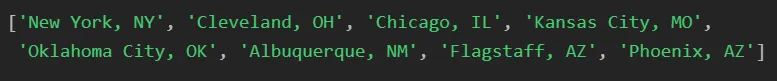
这就是我们数据中从New York, NY到Phoenix, AZ的最短路径!
如果你感兴趣或者想了解更多,可以在这个链接中查看完整的代码。
https://github.com/amos-eda-97/Q-learning-based-optimal-path
作者:Amos Eda